
An independent samples t-test hypothesis test example By Hand
A coffee chain has two locations, one in Queens and one in NYC. The coffee chain owner wants to make sure that all lattes are consistent between the two locations.
A sample of 20 lattes is collected from the Queens store and is determined to have a sample mean of 4.1 oz. of espresso per latte with a sample standard deviation of .12 oz.
A sample of 22 lattes is then taken from the NYC store and is determined to have a sample mean of 4.2 oz. if espresso per latte and a standard deviation of .11 oz.
Use alpha = .05 and run an independent samples t-test to determine if there is a significant difference between the amount of espresso between the two coffee shop lattes.
Step 1: What is Ho and Ha?
Ho: mean espresso in a latte in Queens = mean espresso in a latte in NYC
Ho: mean espresso in a latte in Queens ≠ mean espresso in a latte in NYC
Should you use t-test or z-test and why?
This is best as a t-test because we are comparing two sample means.
Is this a one or two tailed test?
Notice that this is a TWO-TAILED test. We will determine if there is a significant difference.
Our sample size of the Queens sample is n1 = 20 and the std dev s1 is .12
Our sample size of the NYC sample is n2 = 22 and the std dev s2 is .11
Step 2: Calculating the t-test statistic for an independent samples t-test
NOTE: There are three types of t-tests. There is the one sample t-test that compares a single sample to a known population value. There is an independent samples t-test (this example) that compares two samples to each other. There is a paired data (also called correlated data) t-test that compares two samples from data that is related (like pretest score and post test score).
t -test = (sample mean 1 – sample mean 2)/[ sqrt ( s1^2/n1 + s2^2/n2) ]
Recall:
sample mean1 = 4.1, s1 = .12, n1 = 20
sample mean2 = 4.2 , s2 = .11, n2 = 22
NOTE: s1^2 = (.12)^2 = .12 * .12 = .0144
NOTE: s2^2 = (.11)^2 = .11 * .11 = .0121
t -test = (sample mean 1 – sample mean 2)/[ sqrt ( s1^2/n1 + s2^2/n2) ]
t-test = (4.1 – 4.2 ) / [ sqrt (( .12)^2 / 20 + (.11)^2/22) ] =
t-test = (4.1 – 4.2 ) / [ sqrt (.0144 / 20 + .0121/22) ] =
t-test = (4.1 – 4.2 ) / [ sqrt ( .00072 + .00055) ] =
t-test = (4.1 – 4.2 ) / [ sqrt ( .00127 ) ] =
t-test = (4.1 – 4.2 ) / [ .03564 ]
t-test = ( – 0.1 ) / [ .03564 ]
t test = – 2.8058
NOTE: You must use the order of operations when solving any expression.
But – this is not the end of the test!
Step 3: Determine if this value is in a rejection region (reject Ho) or not (do not reject Ho)
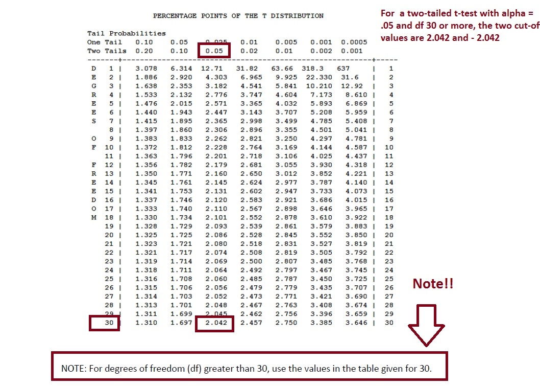
Next, using any t-table (these tables are always on the internet) we can get the critical values (tc) for the two tailed test.
Our degrees of freedom for this one sample t-test is :
df = n1 + n2 – 2 = 20 + 22 – 2 = 40
Our alpha value is .05
Our test is two-tailed
Therefore, using any t-table, the two “critical values” that represent the cut-off points for rejection are:
tc = +/- 2.042
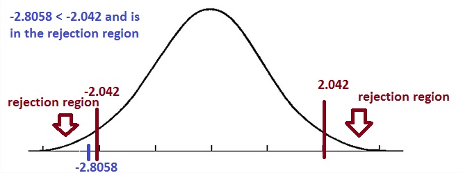
This tells is that if our t-test result (which in this case is 13.6) is either bigger than 2.042 or less than -2.042 then we CAN reject the null because we ARE in the rejection region.
Result:
-2.8058 < – 2.042
Therefore, we must Reject Ho
Step 4: Understanding and writing the conclusion – what does this all mean
Recall that Ho says that there is no sig diff between the lattes in Queens and the lattes in NYC.
However, in this case, we REJECT Ho. Our t-test result WAS in the rejection region because the value was smaller than the cut-off of -2.042. In other words, we do not agree with Ho. We do not think that Ho is correct (with a .05 error margin).
Because we reject Ho (do not choose Ho) we then choose Ha.
Ha tells us that there IS A SIG DIFF between the amount of espresso in the Queens lattes and the amount in the NYC lattes.