A t-test hypothesis test example By Hand

A coffee shop relocates to Italy and wants to make sure that all lattes are consistent. They believe that each latte has an average of 4 oz of espresso. If this is not the case, they must increase or decrease the amount. A random sample of 25 lattes shows a mean of 4.6 oz of espresso and a standard deviation of .22 oz. Use alpha = .05 and run a one sample t-test to compare with the known population mean.

Step 1: What is Ho and Ha?

Ho: mean amount of espresso in a latte = 4 oz
Ha: mean amount of espresso in a latte NOT= 4oz.

 

Should you use t-test or z-test and why?
This is best as a t-test because our sample size is smaller (less than 30) and we know the sample standard deviation, but not the population standard deviation.

Remember: Given any data set, you can always calculate the standard deviation which is the square root of the variance.
Is this a one or two tailed test?

Notice that this is a TWO-TAILED test. However, if the question had asked if the amount is greater or less than, the test would have been different and would have been one-tailed.

It is also possible to run a one-tailed test here because the sample mean is greater than the population mean. However, in this example, we will run the two-tailed test.

Our sample size n = 25.

Step 2: Calculating the t-test statistic (one sample t-test)

NOTE: There are three types of t-tests. There is the one sample t-test that compares a single sample to a known population value (this example). There is an independent samples t-test that compares two samples to each other. There is a paired data (also called correlated data) t-test that compares two samples from data that is related (like pretest score and post test score).

t -test = (sample mean – population mean)/[stddev/sqrt(n)]

The sample mean “x” is 4.6 oz
The “mean” is the population mean of 4 oz.
The sample std dev is .22 oz

n = 25
df = n – 1 = 24
t -test = (sample mean – population mean)/[stddev/sqrt(n)] =(4.6 – 4) / [.22/sqrt(25)]
= (.6)/[.22/5] = .6/.044 = 13.6

Therefore, the t-test value is 13.6

But – this is not the end of the test!

Step 3: Determine if this value is in a rejection region (reject Ho) or not (do not reject Ho)

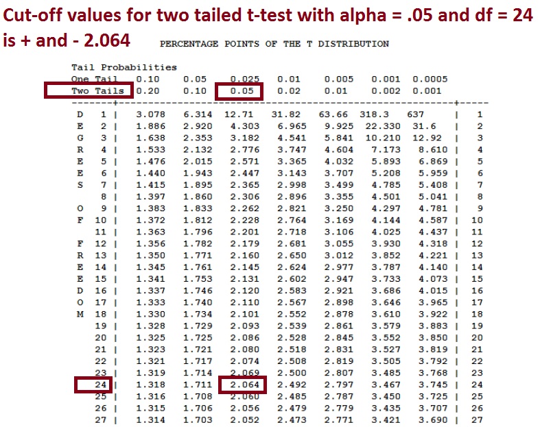
Next, using any t-table (these tables are always on the internet) we can get the critical values (tc) for the two tailed test.

Our degrees of freedom for this one sample t-test is :

df = n – 1 = 25 – 1 = 24

Our alpha value is .05

Our test is two-tailed

Therefore, using any t-table, the two “critical values” that represent the cut-off points for rejection are:

tc = +/- 2.064

This tells is that if our t-test result (which in this case is 13.6) is either bigger than 2.064 or less than -2.064 then we CAN reject the null because we ARE in the rejection region.

Result:

13.6 > 2.064

Reject Ho

 

Step 4: Understanding and writing the conclusion – what does this all mean

Recall that Ho says that there is no sig diff between our sample mean of the amount of espresso in the coffee in Italy and the expected population amount. Ho always says that there is no sig diff.

However, in this case, we REJECT Ho. In other words, we do not agree with Ho. We do not think that Ho is correct (with a .05 error margin).

Because we reject Ho (do not choose Ho) we then choose Ha.

Ha tells us that there IS A SIG DIFF between the amount of espresso in the Italy coffee versus the expected mean.

So – there is too much espresso being placed in the coffee in Italy and it should be reduced to meet the normal (population) mean.